
1 Introduction
From 1875 until 2008 the Northern Hemisphere experienced a temperature increase of 0.79 ºC per century, and the Arctic climate system faced almost double this amount, 1.36ºC per century [Bekryaev, 2010]. The Greenland ice sheet (GrIS) is a key element of the Arctic climatic system. The mass balance of the GrIS is established by two sub-balances: the surface mass balance (SMB) and the liquid water balance. In their model, Van Angelen et al. (2013) calculate a strong increase in melt since 2005, producing low surface mass balance values for the GrIS. The main process behind this recorded mass loss is an increase in melt during the summer period, lowering snow albedo. This yields a higher shortwave radiation (SW) absorption and results in even more meltwater runoff. The runoff increase accounts for more than half of the recent GrIS mass loss [Van Angelen et al., 2013; Van den Broeke et al., 2009].
At intermediate elevations on the GrIS the snow accumulation remains bigger than the melt. The snowfall during the winter compacts the present snow layers, converting them into firn up to 100 m deep [Harper, 2013]. In April 2011 it was discovered that the firn layer of the southeastern GrIS stores liquid water over winter, creating a water body referred to as the perennial firn aquifer (PFA). The amount of liquid water contained in the PFA increases during the melt season. The snow accumulation during winter provides a layer of insulation, preventing the water to refreeze completely [Forster et al., 2013]. It is not fully understood how much of the meltwater stored within the PFA refreezes or contributes to runoff, which creates an uncertainty factor in the mass loss of the GrIS [Harper, 2013; Kuipers Munneke et al., 2014]. Cooling the firn layer requires a significant amount of energy, since the liquid water needs to refreeze before the firn layer can cool down. The projected melt and accumulation increase in the coming years will thus increase the uncertainty of the PFA impact on the GrIS mass and energy 3 balance [Foster et al., 2013; Kuipers Munneke et al., 2014]. This study contributes to a better understanding of the mass loss and the energy balance of the recently discovered PFA area. Using the data of an Automatic Weather Station (AWS) located within this area, the melt during the summer of 2014 is determined using a surface energy balance (SEB) model. Section 2 discusses the specifics of the AWS, the data and the SEB model. Section 3 presents the results, which includes a sensitivity analysis and a comparison with a simulation of a regional atmospheric climate model (RACMO2.3) over the same area.
2 Data and Methods
The data processed for this study are obtained from an AWS in southeast Greenland. Through a computer SEB model, the data is used to calculate the melt. This section provides more information on the measuring location, the data and the SEB model.
2.1 AWS Data
The AWS is an iWS (intelligent weather station for polar use) developed and built at the Utrecht University/Institute for Marine and Atmospheric Research Utrecht (UU/IMAU). It is situated in the PFA area in the southeast of Greenland, 66º22’ N, 39º19’ W, at 1663 m a.s.l. The data were obtained during a period of 238 days, from April 8th, 2014 until December 3rd, 2014, covering the entire melting season. The iWS weighs less, consumes less energy and is more cost-e”cient than a conventional AWS. The iWS continuously records the air temperature (T), relative humidity (Rh), wind speed (U),wind direction (dd), the downward and upwards shortwave and longwave radiative fluxes (SWin and LWin, SWout and LWout) and 4 snow height variations, and relays the data to the UU/IMAU by satellite. Table 1 provides an overview of the specific sensors used, their accuracy and range.
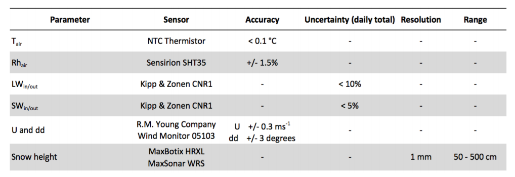
Table 1: An overview of the iWS sensors, the parameters they measure, their accuracy and range. Note: the CNR1 has shown to be more accurate than indicated by the manufacturer [Van den Broeke et al., 2004].
The iWS experienced minor offsets in its observations, resulting in data errors which have been corrected as follows. The air temperature sensor is placed inside a radiation screen which is naturally ventilated, typically resulting in measurement errors under conditions of high SWin and low U (radiation errors). A thin wire thermocouple of minimal thickness acts as reference for the temperature correction. The relative humidity sensor is positioned under the iWS housing inside a filter cap; the data are of high quality, since Rh is measured at the same chip as Tair. The longwave radiation sensors experienced a measuring error due to solar radiation absorption by its window, which is transferred to the sensors. This window heating can result in an error up to 20 W m”2 on a sunny day (SWin ⇠ 1000 W m”2) with low wind speeds. This was corrected using the outgoing radiation of the snow surface during melt periods when LWout should be constant at 315 W m”2. The corrections for both LWin and LWout are performed by fitting SWout to (LWout, measured ” LWout, melting snow).
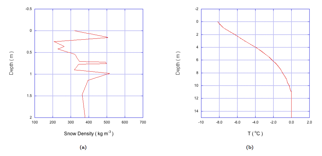
Fig. 1: (a) The initial snow density profile and (b) the initial subsurface temperature.
The density of the snowpack was measured at the beginning of the measurement period using a small mechanical drill. It has been interpolated to obtain the initial snow density profile as a function of the snow depth (Figure 1a). Past 2 m depth, the snow density is taken to be constant at ⇢snow= 380 kg m”3. The initial subsurface temperature profile of the snowpack is presented in Figure 1b. 2.2 SEB Model The melt energy of the snowpack is determined by the surface energy balance (SEB), defined as

all elements in units [W m”2]. SWnet represents the net shortwave radiation, LWnet the net longwave radiation, Hsen the turbulent sensible heat flux, Hlat the turbulent latent heat flux, G˜s the subsurface heat flux at the surface and M the melt energy. This is the same SEB model as used and described in Kuipers Munneke and others (2012). The time steps of the model are set to 150 seconds, ande the layer thickness to 2 cm. The coming subsections will briefly describe the different components of the model.
2.2.1 Radiative Fluxes
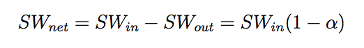
The net shortwave radiation is determined by SWin and the surface albedo, ↵, the fraction of the incoming shortwave radiation that is reflected by the surface. The net shortwave radiation is then calculated as follows:
Radiative energy is emitted by the earth’s surface as thermal longwave radiation, LWout, which is absorbed by the lower atmosphere. This longwave radiation is emitted again by the atmosphere, partially directed towards the earth’s surface, described by LWin. These parameters can be calculated with the Stefan Boltzmann law for natural surfaces
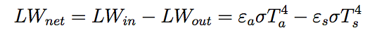
where $ represents the Stefan Boltzmann constant, εa and εs the (effective) emissivity of the atmosphere and surface respectively (for a blackbody, ε = 1), Ta and Ts the temperature of the atmosphere and surface respectively. The radiation balance is then determined by:
Note that all radiative fluxes are measured.
2.2.2 Turbulent Fluxes
The two surface turbulent fluxes in the energy balance are Hsen and Hlat. The sensible heat flux describes the vertical turbulent transfer of heat between the surface and the atmosphere. The flux is determined through
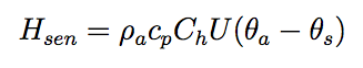
where ⇢a represents the air density calculated using p = ⇢RaT (1.25 kg m”3), cp the specific heat of air (1004 J kg”1 K”1) , Ch the bulk turbulent heat exchange coe”- cient, U the wind speed and ✓a and ✓s the potential temperatures in the atmosphere and at the surface respectively. The latent heat flux is the vertical turbulent latent heat exchange through moisture transport, e.g. evaporation/sublimation and condensation/riming, and is given by
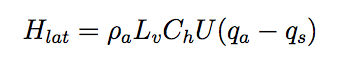
where Lv denotes the latent heat for vaporisation/sublimation (2.50⇥10^6/2.83⇥10^6 J kg^-1) and (qa – qs) the difference in specific humidity between the atmosphere and the surface.
2.2.3 Subsurface Heat Fluxes
G describes the vertical conductive energy flux below the surface. This vertical energy flux results from heat exchange between different layers within the subsurface, which is dependent on the snow density profile. G is given by where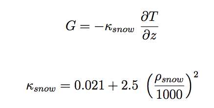
represents the thermal conductivity of snow, which depends on the snow density [Anderson, 1976]. Its surface value (Gs) is determined by the surface density and temperature gradient. In this study, both subsurface heat fluxes and subsurface solar radiation penetration (Q) are combined in the parameter G˜s, because the snowpack heats up quicker than expected from the subsurface heat flux by itself. The subsurface heat flux presented above thus does not distinguish between changes in the snow’s heat capacity due to diffusion or solar radiation absorption by the subsurface. This model determines the radiation penetration which occurs in the first 10 cm in the snow, by layers of 2 mm [Kuipers Munneke et al., 2012].
2.2.4 Roughness Length
The surface roughness length z0 determines the distance from the surface at which the wind speed extrapolates to zero. It is related to the size of the surface roughness elements; its value is assumed to be constant at the value of snow, which is taken to be z0,snow = 1.26⇥10″1 m in this study.
2.3 RACMO2.3
RACMO2.3 is the Regional Atmospheric Climate Model of the Royal Netherlands Meteorological Institute (KNMI) [Van Meijgaard et al., 2008]. It uses a combination of the physics module from the European Centre for Medium-Range Weather Forecasts Integrated Forecast System (ECMWF-IFS) and the atmospheric dynamics from the High Resolution Limited Area Model (HIRLAM). The IMAU has developed a polar version dedicated to the simulation of the GrIS SMB, by adding a snow module. This added module e.g. relates the snow albedo to the size of snow grains, allowing for more accurate meltwater estimations. The snow module also simulates the runoff and refreezing of the meltwater [Ettema et al., 2010]. RACMO2.3 uses a grid resolution of 11 km with 40 vertical atmospheric layers [No¨el et al., 2015]. Section 3.4 discusses the correspondence between the data obtained from RACMO2.3 and the output of the SEB model.
3 Results
This section presents the melt calculated by the SEB model. The different components of the SEB are discussed, including a sensitivity analysis. Lastly, a comparison is made with the SEB of the RACMO2.3 simulation of the same location.
3.1 Meteorology
This subsection provides a brief overview of the meteorology during the melting season of 2014. The mean air temperature was -8.2 ºC, with a maximum of 6.6 ºC and a minimum of -27 ºC. On May 19th, positive temperatures were recorded for the first time for a short period only. Between June 10th and August 24th temperatures above zero were observed constantly during daytime. After a short period of continuous frost, the last positive temperatures were recorded on September 2nd. The daily average temperatures are shown in Figure 2a. The average wind speed was 6.1 m s”1, and the daily means are plotted in Figure 8b. There is an evident correlation between high wind speeds and low air temperatures. The specific humidity, Figure 2c, varies in accordance with the temperature of the air. The air at this location was rather moist, with a mean relative humidity of 89%.
3.2 SEB
The SEB model closes the energy balance in Eq. (1) by looking iteratively for the correct surface temperatures. Using this computed temperature (Tcalc) it is possible to verify the accuracy of the model, by comparing it with the temperature
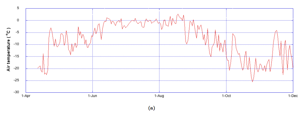
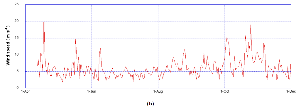
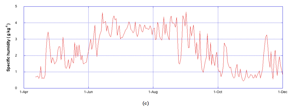
Fig. 2: (a) Daily mean of the air temperature, (b) wind speed and (c) specific humidity.
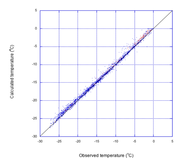
Fig. 3: A scatterplot with the observed surface temperatures and the modelled surface temperatures, as a performance verification for the SEB model. The blue dots represent the hourly values, the red dots the daily means. deduced from the outgoing longwave radiation (Tobs). Figure 3 provides a scatterplot of these two quantities. The mean difference between these parameters is 0.39 ºC, with a RMSE of 0.95 ºC for hourly data. For daily averages the mean difference is the same, but the RMSE reduces to 0.54 ºC. Differences mainly occur at low temperatures, likely caused by a measurement offset in the longwave radiation. In any case, the model shows a good performance.
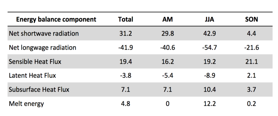
Table 2: The total and the seasonal average of the SMB components. All values denoted in [W m”2].
Table 2 provides an overview of the total and the seasonal averages of the SEB components discussed in Section 2. The daily means of the SEB components are presented in a bar diagram in Figure 4. During summer, the net shortwave radiation increases and so does the sensible heat flux. The net longwave radiation and the latent heat flux decrease, but to a lesser extent. This yields a positive energy balance, which is restored by contributing energy to melt. The net shortwave radiation decreases significantly in fall notably after a snowfall event in late August with cloudy conditions, and the net longwave radiation increases. This also induces a drop in the subsurface heat flux because the radiation penetration is reduced. Lastly, the latent heat flux experiences some positive values after summer, when atmospheric moisture increases.
The total melt is determined by the sum of the surface and the subsurface melt. During summer 2014 the total cumulative melt was 537 kg m”2. The surface and subsurface melt both contribute approximately equally. Without the radiation penetration module discussed in Section 2.2.3 the subsurface melt does not contribute to the total melt. This yields a total melt of 475 kg m”2, thus
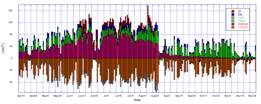
Fig. 4: The daily mean of the SEB fluxes.
an underestimation of over 10%. Figure 5 shows the evolution of the cumulative total melt and the water content of the snowpack, combined with the runoff and refreezing. Since part of the meltwater refreezes in the beginning of the melt season, the water content does not increase equally quickly with the melt. At the end of July, temperatures above zero appear more frequently and for longer periods. Refreezing has warmed the snow, and this results in a decrease of melt water refreezing and more water is contributed to runoff, reducing the water content of the snow pack. After September 2nd melting ceases and through refreezing the water content gradually decreases. The snow height is initialised at the iWS’ initial distance to the surface (3 m). Figure 6 presents the evolution of the height of the snowpack over time, together with the melt energy. As temperatures rise towards summer and melt occurs, the snow height decreases. During a short period of snowfall and frost at the end of June the snowpack accumulates, to again drop slightly below its initial height at the end of the summer. However, at the end of August accumulation occurs again and towards the winter the snowpack quickly thickens. The mean daily
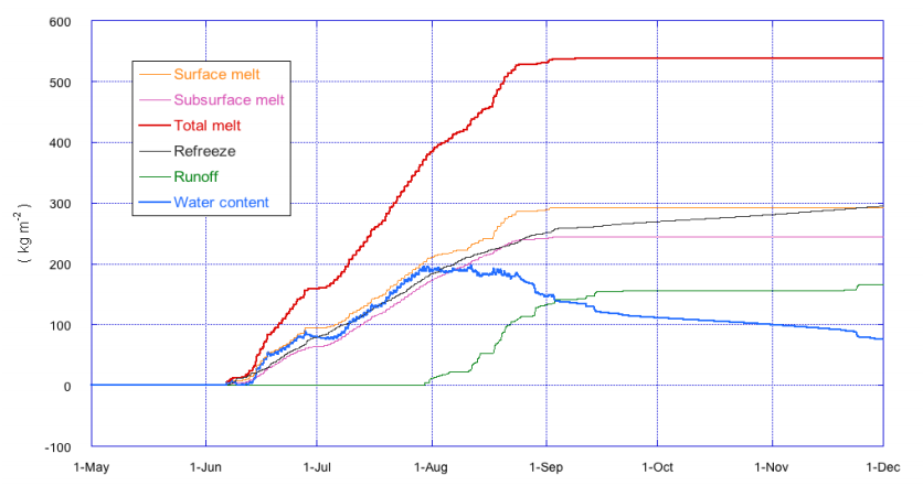
Fig. 5: The total melt is presented as a sum of the surface and the subsurface melt, and is plotted against the water contained within the snowpack. All parameters are cumulative. Note that sublimation and rime (contributing negatively to the water content) are not plotted in this diagram.
average albedo is presented in Figure 7. A low albedo results in high net shortwave radiation accommodating melt. As fresh snow increases the surface’s reflectivity, the albedo increases after snow accumulation. This is in good correspondence with a minimum albedo of 0.72 during summer and a maximum of 0.95 after snowfalls. Even though the change in snow height seems in correspondence with the melt, the melting period and the albedo, it must be noted that there remains a discrepancy. The sonic height ranger does not have a fixed reference point on the surface and cannot be concluded which snow layer is melting or whether the observed height change is due to e.g. compaction. In the absence of density observations, this remains a factor of uncertainty [Kuipers Munneke et al., 2012].
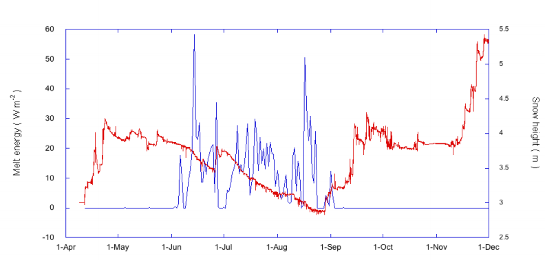
Fig. 6: The snow height plotted against the daily mean melt energy. The height of the snow was initialised at 3 m.
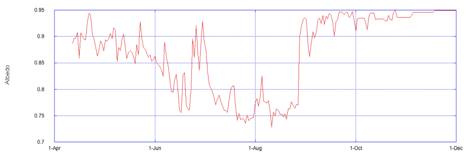
Fig. 7: The daily mean albedo.
3.3 Sensitivity Analysis
This sensitivity analysis assesses the sensitivity of the SEB components to changes in input parameters of the model. The results are presented in Table 3. The reference is the optimal run, used for the results presented above. Only the component indicated is changed.
Upon increasing the air temperature by 1 ºC, the model preforms less accurately, indicated by the RMSE and the mean error. There is an increase in the turbulent fluxes as the vertical heat transfer grows. The total melt rises significantly by the increase of longwave radiation. An increase in the windspeed of 0.5 m s^-2 does only alter the results insignificantly. However, Section 2.2.2 shows that the absolute values of the turbulent fluxes are amplified. The relative humidity is closely related to the latent heat flux. As it increases by 5%, the latent heat flux increases, as more moisture can be released to the surface. The melt is expected to increase noticeably. The surface roughness lengths show an interesting behaviour, since an increase yields a much bigger effect than a decrease by the same factor. The effects are, however, opposite. The higher sensitivity for an increase results in a bigger difference between the turbulent fluxes, providing more melt energy.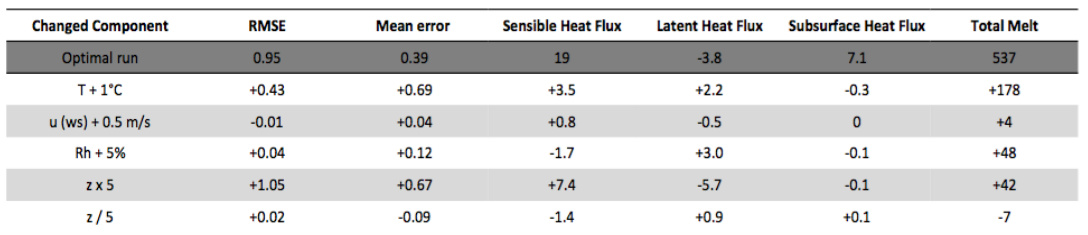
Table 3: The sensitivity analysis, presenting the effect of a change in parameters of the model on the SEB components. Only one parameter is changed per run. The RMSE and mean error are in units [ºC], the fluxes in [W m^-2] and the total melt in [kg m^-2]. The optimal run is the data used in this study.
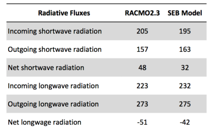
Table 4: The mean values of the radiative components of the RACMO2.3 and the SEB model data. All values are determined using daily means, all in [W m”2].
3.4 RACMO2.3 Simulation
In order to assess the performance of RACMO2.3, two adjacent pixels are evaluated with the obtained iWS data. The first pixel covers the area around the iWS site, referred to as Y0, at an elevation of 1672 m a.s.l. As this exceeds the elevation of the iWS a second adjacent pixel with a more similar elevation of 1664 m a.s.l., Y-1, is evaluated too. Figure 8a shows the temperatures simulated by RACMO2.3 of both pixels and the observed temperature. The differences between the observed temperatures and the RACMO2.3 temperatures are plotted in Figure 8b. The RMSE between Tobs and TY 0 is 1.72 ºC with a mean error of 0.45 ºC. Between Tobs and TY ^-1 these values are 1.60 ºC and 0.23 ºC respectively. The second pixel is in better correspondence with the observations and will be used as reference for the coming analysis.
Table 4 shows the mean values of the radiative fluxes for both data sets. Figure 9 presents some of the differences in SEB components and parameters between the RACMO2.3 simulation (blue) and the SEB model (red). Figure 9a shows that
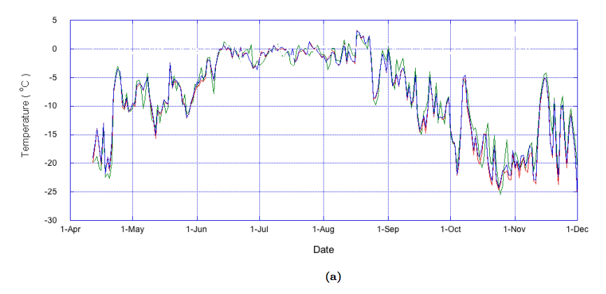
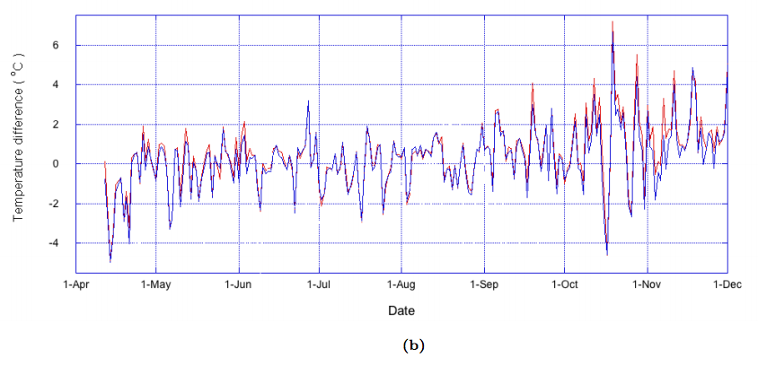
Fig. 8: (a) The absolute temperature of Y0 (red), Y-1 (blue) and the observed temperature (green), and (b) the difference of the observed temperature with the simulated temperatures in RACMO2.3 for both pixels. Y-1 (blue) yields a lower mean difference than Y0 (red).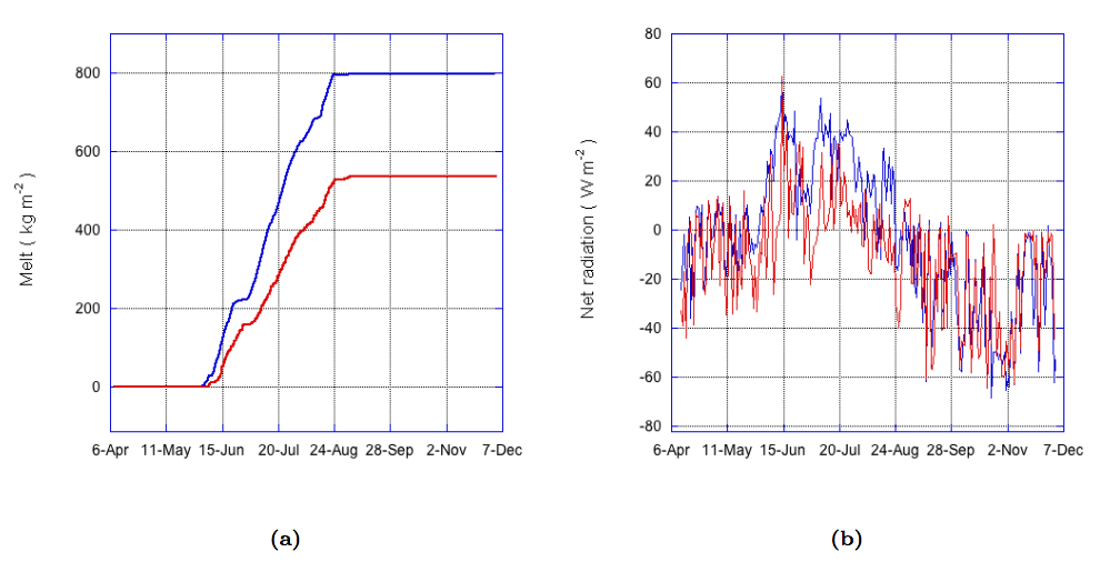
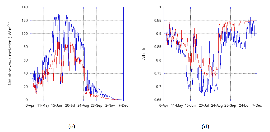
Fig. 9: Comparison of the data output between the SEB model (red) and the RACMO2.3 simulation (blue) for (a) the melt, (b) the radiation balance, (c) the net shortwave radiation and (d) the surface albedo. the data of the RACMO2.3 simulation determines the melt almost 260 kg m”2 higher than the SEB data. The net radiation is shown in Figure 9b, and during the melt period RACMO2.3 yields a consistently higher radiation balance. Figure 9c shows that this offset originates partially from a higher net shortwave radiation in RACMO2.3. Table 4 shows that the net longwave radiation is underestimated, amplifying the net radiation offset. Overall, however, the mean values of the radiative fluxes show no substantial differences. The albedo in RACMO2.3 almost continuously takes lower values than modelled for the SEB (Figure 9d), explaining the melt overestimation.
There are several possible explanations for the low surface albedo simulated by RACMO2.3, resulting in higher melt. A first logical explanation would be a difference in modelled cloud cover. The cloud cover of RACMO2.3 was not available for this run. Yet, since the cloud cover is related to the incoming longwave radiation, these components can be compared. Table 4 shows only a small discrepancy between the incoming longwave radiation modelled by the SEB and RACMO2.3. This makes cloud cover less likely to be causing the offset. Another possible cause is an underestimation of precipitation by RACMO2.3. Research has shown that RACMO2.3 often underestimates the precipitation in accumulation zones by 25 mm [No¨el et al., 2015]. Melt wets the snow, which makes it darker, yielding a decrease in surface albedo. However, precipitation can deposit new snow layers, restoring the high albedo. In Figure 9 it can be observed that during periods of melt, the RACMO2.3 albedo decreases too quickly. Yet, after an episode of snow the albedo is restored to higher values. Another factor affecting the snow albedo negatively is impurity content in the form of black carbon. Black carbon in snow is known to increase the radiative forcing significantly, magnifying the melt. It is thus likely that RACMO2.3 overestimates the albedo during melt due to an overestimation of black carbon content [Van Angelen et al., 2012]. As a result, the albedo is consistently lower, resulting in a significantly higher total melt at the end of summer.
As explained before, RACMO2.3 contains a snow module which models the properties of the snow pack. The surface albedo is also determined in this module, creating a dependence on properties such as grain size and water content. In the SEB model the albedo is only determined using the incoming and reflected solar radiation. The difference in nature of these calculations certainly plays a role in the observed offset. Moreover, the sonic height ranger is the main indicator of precipitation for the iWS. However, as discussed in Section 3.2, these observations are too uncertain to draw a conclusion. For certainty about the cause of the difference in expected melt between the two data sets, more accurate measurements of precipitation and snow depth are needed. Adding to this, a complete mass balance would be required in order to gain further insight in this aspect. Hence, this remains a point of discussion for this study.
4 Discussion and Conclusions
The SEB within the PFA area of the eastern GrIS is calculated using a model that fits skin temperatures to the balance in order to close it. The RMSE between the observed and the modelled hourly (daily) temperatures is 0.95 ºC (0.54 ºC). As this difference is within the uncertainty of the longwave radiation sensor, the model shows an accurate performance. The total melt over the summer of 2014 is calculated to be 537 kg m^-2. In order to determine the subsurface melt, the subsurface heat flux included heating due to the absorption of solar radiation. The use of this radiation penetration module prevented an underestimation of the melt higher than 10%. Kuipers Munneke (2009) suggests two additional methods of verifying the model’s performance. Firstly, through comparing the modelled and the measured sensible heat flux. However, the iWS was not equipped with a sonic anemometer making such data not available as a reference point. Secondly, through the evolution of the subsurface temperature modelled and measured. This has also not been used as an input parameter for the model as the sensor depth was not calibrated with the changing height of the snowpack.
A comparison was made between the data of a RACMO2.3 simulation and the output data of the SEB model. Even though the temperatures were corresponding accurately (mean error 0.23 ºC), there was a significantly higher estimation for total melt of over 260 kg m”2 by the RACMO2.3 data. The cause of this was the difference in surface albedo during the melt period. RACMO2.3 uses prescribed snow properties to determine the albedo, whereas the SEB model only uses the sum of the incoming and reflected solar radiation, creating discrepancies. RACMO2.3 may underestimate precipitation, which increases snow ageing and thus lowers the albedo. Alternatively, the prescribed impurity content is too high. However, in order to assess this more carefully, a surface mass balance is required.
Further understanding of the behaviour of water content in the snowpack and related parameters such as runoff and refreezing is needed in order to diminish the uncertainty factor of the PFA. This requires modelling of the snow properties and calculating a full mass balance. As presented, the SEB model displays the water content, runoff and refreezing, showing the rough behaviour of liquid water in the snowpack over the melt period. This gives a first understanding of these aspects. The SEB presented in this study, however, gives insight in the magnitude and behaviour of the fluxes in the PFA area from on-site observational data.
Bibliography
Anderson, E. A. (1976). A point of energy and mass balance model of snow cover. Tech. Rep. NWS19, NOAA.
Bekryaev, R., Polyakov, I., & Alexeev, V. (2010). Role of Polar Amplification in Long-Term Surface Air Temperature Variations and Modern Arctic Warming. Journal Of Climate, 23(14), pp. 3888-3906. http://dx.doi.org/10.1175/2010jcli3297.1
Ettema, J., van den Broeke, M. R., van Meijgaard, E., van de Berg, W. J., Box, J. E., & Steffen, K. (2010). Climate of the Greenland ice sheet using a highresolution climate model ? Part 1: Evaluation. The Cryosphere, 4, pp. 511?527. doi:10.5194/tc-4-511-2010
Forster, R., Box, J., van den Broeke, M., Mige, C., Burgess, E., & van Angelen, J. et al. (2013). Extensive liquid meltwater storage in firn within the Greenland ice sheet. Nature Geoscience, 7(2), pp. 95-98. http://dx.doi.org/10.1038/ngeo2043
Harper, J. (2013). Cryosphere: Greenland’s lurking aquifer. Nature Geoscience 7(2), pp. 86-87. http://dx.doi.org/10.1038/ngeo2061
Kuipers Munneke, P., van den Broeke, M., King, J., Gray, T., & Reijmer, C. (2012). Near-surface climate and surface energy budget of Larsen C ice shelf, Antarctic Peninsula. The Cryosphere, 6(2), pp. 353-363. http://dx.doi.org/10.5194/tc-6-353-2012
Kuipers Munneke, P., M. Ligtenberg, S., van den Broeke, M., van Angelen, J., & Forster, R. (2014). Explaining the presence of perennial liquid water bodies in the firn of the Greenland Ice Sheet. Geophys. Res. Lett., 41(2), pp. 476-483. http://dx.doi.org/10.1002/2013gl058389
Noël, B., van de Berg, W., van Meijgaard, E., Kuipers Munneke, P., van de Wal, R., & van den Broeke, M. (2015). Evaluation of the updated regional climate model RACMO2.3.3: summer snowfall impact on the Greenland Ice Sheet.The Cryosphere, 9(5), pp. 1831-1844. http://dx.doi.org/10.5194/tc-9-1831-2015
Van Angelen, J., Lenaerts, J., Lhermitte, S., Fettweis, X., Kuipers Munneke, P., & van den Broeke, M. et al. (2012). Sensitivity of Greenland Ice Sheet surface mass balance to surface albedo parameterization: a study with a regional climate model. The Cryosphere, 6(5), pp. 1175-1186. http://dx.doi.org/10.5194/tc-6- 1175-2012
Van Angelen, J., van den Broeke, M., Wouters, B., & Lenaerts, J. (2013). Contemporary (1960-2012) Evolution of the Climate and Surface Mass Balance of the Greenland Ice Sheet. Surv. Geophys., 35(5), pp. 1155-1174. http://dx.doi.org/10.1007/s10712-013-9261-z
Van den Broeke, M., van As, D., Reijmer, C., & van de Wal, R. (2004). Assessing and Improving the Quality of Unattended Radiation Observations in Antarctica. J. Atmos. Oceanic Technol., 21(9), pp. 1417-1431. http://dx.doi.org/10.1175/1520-0426(2004)021¡1417:aaitqo¿2.0.co;2
Van den Broeke, M., Bamber, J., Ettema, J., Rignot, E., Schrama, E., & van de Berg, W. et al. (2009). Partitioning Recent Greenland Mass Loss. Science, 326(5955), pp. 984-986. http://dx.doi.org/10.1126/science.1178176
Van Meijgaard, E., van Ulft, L. H., van de Berg, W. J., Bosveld, F. C., van den Hurk, B., Lenderink, G., & Siebesma, A. P. (2008). Technical Report 302: The KNMI regional atmospheric climate model RACMO version 2.1. Royal Netherlands Meteorological Institute, De Bilt.
List of Figures
1 Two numerical solutions . . . . . . . . . . . . . . . . . . . . . . . . 6
2 Two numerical solutions . . . . . . . . . . . . . . . . . . . . . . . . 11
3 A scatterplot with the observed surface temperatures and the modelled surface temperatures, as a performance verification for the SEB model. The blue dots represent the hourly values, the red dots the daily means. . . . . . . . . . . . . . . . . . . . . . . . . . . . . . 12
4 The daily mean of the SEB fluxes. . . . . . . . . . . . . . . . . . . . 14
5 The total melt is presented as a sum of the surface and the subsurface melt, and is plotted against the water contained within the snowpack. All parameters are cumulative. Note that sublimation and rime (contributing negatively to the water content) are not plotted in this diagram. . . . . . . . . . . . . . . . . . . . . . . . . 15
6 The snow height plotted against the daily mean melt energy. The height of the snow was initialised at 3 m. . . . . . . . . . . . . . . . 16
7 The daily mean albedo. . . . . . . . . . . . . . . . . . . . . . . . . . 16
8 (a) The absolute temperature of Y0 (red), Y-1 (blue) and the observed temperature (green), and (b) the difference of the observed temperature with the simulated temperatures in RACMO2.3 for both pixels. Y-1 (blue) yields a lower mean difference than Y0 (red). 19
9 Comparison of the data output between the SEB model (red) and the RACMO2.3 simulation (blue) for (a) the melt, (b) the radiation balance, (c) the net shortwave radiation and (d) the surface albedo. 20
List of Tables
1 An overview of the iWS sensors, the parameters they measure, their accuracy and range. Note: the CNR1 has shown to be more accurate than indicated by the manufacturer [Van den Broeke et al., 2004]. 5
2 The total and the seasonal average of the SMB components. All values denoted in [W m”2]. . . . . . . . . . . . . . . . . . . . . . . 13
3 The sensitivity analysis, presenting the effect of a change in parameters of the model on the SEB components. Only one parameter is changed per run. The RMSE and mean error are in units [ºC], the fluxes in [W m^-2] and the total melt in [kg m^-2]. The optimal run is the data used in this study. . . . . . . . . . . . . . . . . . . . . . 17
4 The mean values of the radiative components of the RACMO2.3 and the SEB model data. All values are determined using daily means, all in [W m^-2]. . . . . . . . . . . . . . . . . . . . . . . . . . 18